1. Introduction to Python and Jupyter Notebooks¶

This lesson will give a short introduction on how to work with Notebooks in combination with Python. It consists of explanation followed by pratical exercises. To get the most out of this lesson it is best to manually type the code into your Jupyter Notebook instead of copy-pasting.

Notebooks¶

First, lets start up Jupyter and open a Notebook. In the taskbar searchbox, type ‘jupyter’ and open jupyter notebook.

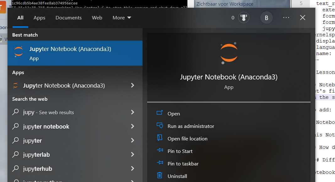
Fig. 1 Open Jupyter Notebook.¶

This should open a tab in your browser with the jupyter hub in the installation folder. This folder will act as your home folder for jupyter. All Notebooks you make will be stored here unless explicitely saved elsewhere or moved.

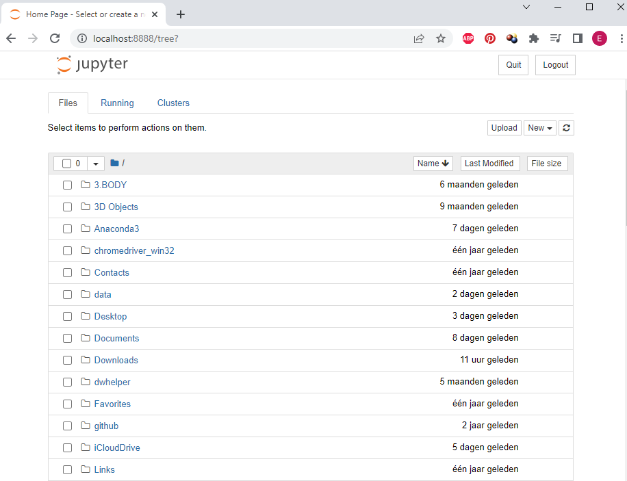
Fig. 2 The Jupyter home or hub where all Notebooks reside.¶

To open a new Python Jupyter Notebook click the new button in the topright corner and select python3 from the dropdown list.

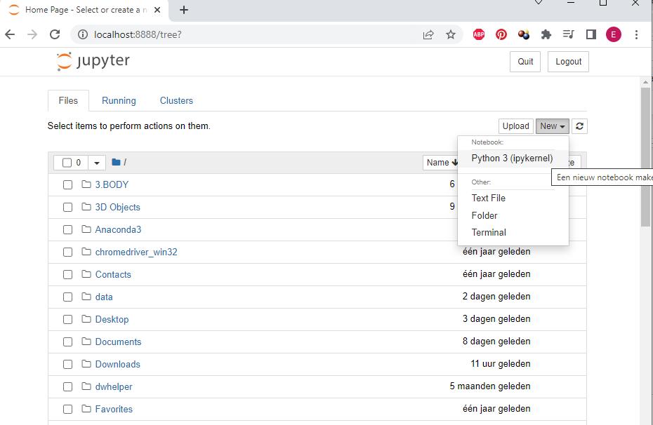
Fig. 3 Click new and python3 to open a new Notebook.¶

A new tab should open dispaying your new Notebook, usually called Untitled

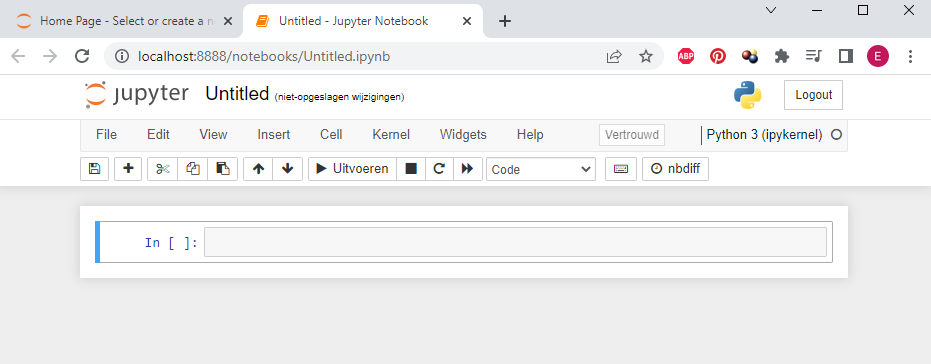
Fig. 4 Your freshly started Notebook with inspiring name.¶

Notebooks can be renamed by clicking on the name and typing a different name. It is best to make these names descriptive so they are still recognizable after a while.

How does a Notebook work?¶

A Notebook is not a static page, but an interactive enviroment. Within the blocks (cells) of a Notebook code can be written ánd executed.

Different cell types¶

Notebooks are compromised of different types of cells. The main cell types are text cells and code cells.

Text cells are generally used for descriptions and explanations. These cells are inactive and code written in these cells cannot be executed.

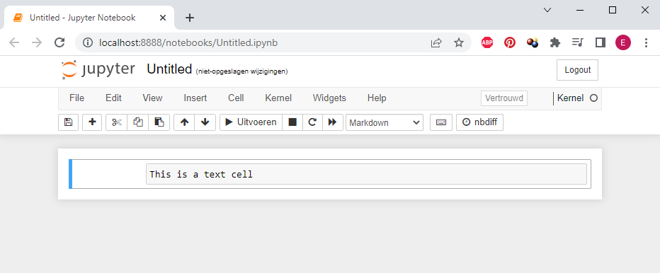
Fig. 5 This is a text cell.¶

The layout is managed through markdown (see markdown syntax for more information).

The second main type of cell is the code cell. Code cells are used to write and execute code. In our case Python. When a code cell is run, Python will execute the code in the cell. More information about Python will follow in the next section.

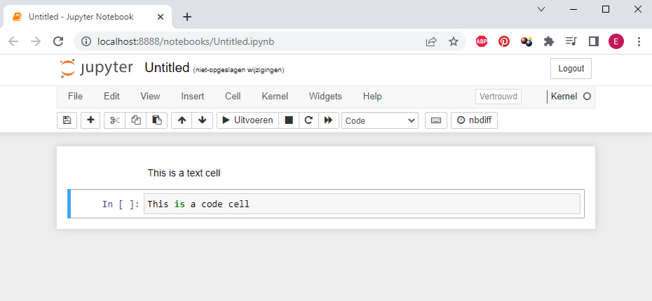
Fig. 6 This is a code cell.¶

Code cells are easily recognized by the ‘In [ ]:’ to the left of the cell.

The type of a cell can be changed by selecting a cell and either going through the menu (Cell/Cell Type/

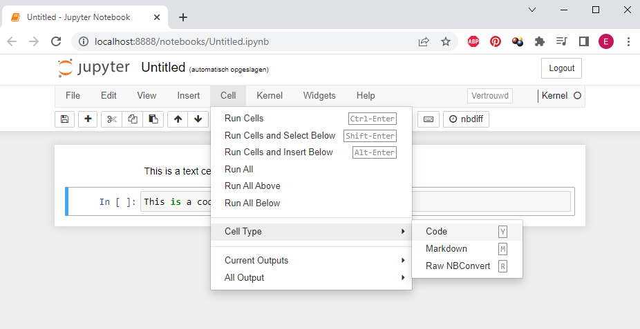
Fig. 7 Via this menu you can select the cell type.¶

Exercise

Select a cell in the Notebook and change the type by using the hotkeys or the menu.

Running cells¶

There are multiple ways to run a cell:

By clicking the ‘Run’ button in the taskbar;
By pressing ‘shift + enter’ when the cell is selected (green frame) Note that this will move the selection box down one cell. When the end of the cells is reached this will add new empty cells to the Notebook.

The moment a cell generates output the output is displayed beneath the cell, keeping code and output together.

Exercise

Type the code below in a new code cell in your Notebook and run the cell.

2*8

Solution

Python will simply multiply the numbers and display the answer below the code cell.

Adding new cells¶

One cell is rarely enough to make a clearly structured Notebook. Adding more cells can be done by pressing the ‘+’ button in the taskbar.

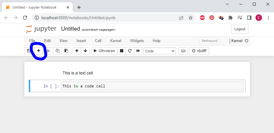
Fig. 8 Click the + to add a new cell directly below the selected one¶

This will add a new cell directly below the currently active cell.

Another way is to use the menu ‘Insert’, where the choice is given between adding a cell above or below the current active cell.

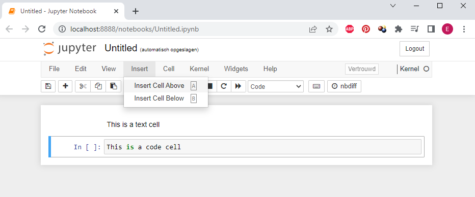
Fig. 9 In this menu you can add a new cell above or below.¶

Comments¶

Comments can be added to a code cell. Comments can be used to describe what a piece of code does, or can be used to tell where values can be changed.

# This is an example of a comment in a code cell.

The moment a # is typed in a code cell, everything after it on the same line will be regarded as a comment. Lines that have been marked as a comment will not be executed by Python when the cell is run.

Exercise

Type the code below in a new cell in your Notebook and run the cell. Does Python return output?

#print("The solution to 35+12 is:")
#print(35+12)

Solution

The cell should not return any output as the code is commented out by the #.

When the # is removed and the cell is run again, Python wil recognize the code and execute it.

Exercise

Alter the cell so the code is no longer seen as a comment.

Solution

Removing the # from the code should enable Python to recognize the code and return output when the cell is run.

print("The solution to 35+12 is:")
print(35+12)

This should then print:

The solution to 35+12 is: 
47

Python¶

Python was developed in 1991 by Guido van Rossum. The purpose of Python was to create a programming language that is both simple to understand and readable. Python works on different platforms such as Windows, Mac, Linux, etc. It is a very popular programming language in data analysis and data science because of its versatality. Python is open source, and can therefore be used for free.

Input and variables¶

When using Python there are multiple types of input data, such as lists, numbers, text, and even whole tables. We put these input into variables. A variable is essentially a container for the data. The name of a variable is up to your own discretion, although there are some rules and guidlines. Python remembers which input was loaded into which variable. This means that the variables can be used in the code instead of the data itself.

When creating a variable, it is important to input data correctly: for numbers no quotation marks are used, for text quotation marks must be used!

The command type() can be used to determine what type of input a variable contains. For example: int indicates a variable contains an integer, or whole number. str indicates a variable contains a string, a piece of text.

Exercise

Type the code below in a newcell in your Notebook and run the cell.

# This stores the data in the variable
number = 9
# This determines its type
type(number)

Solution

Python will return the type of the variable.

int

Now let’s repeat that for another data type.

Exercise

Type the code below in a new cell in your Notebook and run the cell.

# This stores the data in the variable
text = "this is a text"
# This determines its type
type(text)

Solution

Python will return the type of the variable.

str

Note

Important! If you input a number with quotation marks Python will see it as text!

Exercise

Type the following code in a new cell in your Notebook and run the cell. What data type is the number?

number_but_wrong = "9"
type(number_but_wrong)

Solution

The cell should return ‘str’. The number is seen as a string because of the quotation marks.

Note

Sometimes an error in the code is due to the wrong data type. Checking data type is always a good start when error checking.

As mentioned above it is possible to use previously assigned variables in your code. This makes it possible to input a value just one time when it is needed more than once in the code.

Exercise

Type the code below in a new cell in your Notebook and run the cell.

number_1 = 3
number_2 = 6

number_1 + number_2 

Solution

Python simply adds the original numbers as it remembers which input belongs to which variable.

Exercise

Using Python variables, calculate the sum of “35 + 69” in the cell below. Start with making two variables to assign the numbers 35 and 69 to. Calculate the sum using these variables.

# Make a variable for the number 35

# Make a variable for the number 69

# Calculate the sum using the variables

Solution

Your code should look a bit like this:

number_1 = 35
number_2 = 69
number_1 + number_2 

The plus sign can be used to calculate sums, as you did in the above exercise. However, the plus sign can also be used to stick different strings together.

Exercise

Type the code below in a new cell in your Notebook and run the cell.

line_1 = "This is a "
line_2 = "stuck together text"
line_1 + line_2

Solution

As you can see Python adds the text elements together to form a longer sentence. This also works with multiple variables.

'This is a stuck together text'

Exercise

Ensure that the four lines below are printed as one sentence in the output.

line_1 = "Because of this Notebook "
line_2 = "I now know "
line_3 = "that programming with Python "
line_4 = "is very fun!"

Solution

Your code should look like this:

line_1 + line_2 + line_3 + line_4

'Because of this Notebook I now know that programming with Python is very fun!'

Now, what about adding text and numbers from variables together?

Exercise

Type the code below in a cell in your Notebook and see what happens when you run the code.

line_1 = "The amount of abstracts for DHBenelux is: "
amount_1 = 43
line_1 + amount_1

Solution

This gives an error:

TypeError: can only concatenate str (not "int") to str

Just adding numbers and text does not work. Some extra work needs to be done in order for Python to correctly return output without errors

---------------------------------------------------------------------------
TypeError                                 Traceback (most recent call last)
Input In [10], in <cell line: 3>()
      1 line_1 = "The amount of abstracts for DHBenelux is: "
      2 amount_1 = 43
----> 3 line_1 + amount_1

TypeError: can only concatenate str (not "int") to str

There are multiple options to convince Python to return combinations of numbers and text:

force numbers to text with str()
f strings

To force Python to interpret a number as text its type can be changed with str(number).

Exercise

Type the code below in a new cell in your Notebook and run the cell.

line_1 = "The amount of abstracts for DHBenelux is: "
amount_1 = 43
line_1 + str(amount_1)

Solution

Now the text and number are succesfully stuck together.

```{code-cell} 
:tags: [remove-output,hide-output]
line_1 = "The amount of abstracts for DHBenelux is: "
amount_1 = 43
line_1 + str(amount_1)

This also works with multiple variabeles and pieces of text outside of variables.

Exercise

Type the code below in a new cell in your Notebook and run the cell.

line_1 = "coffee breaks "
amount_1 = 2
 
"The amount of " + line_1 + "in this workshop is: " + str(amount_1)

Solution

Python will stick anything together, as long as it is of type text.

'The amount of coffee breaks in this workshop is: 2'

Note

Notice the space after each of the pieces of text (either in or outside a variable). Try removing it to see what happens

Another option is the use of f strings. This is a way of telling Python where to insert the contents of a variable into a string.

The syntax for f strings is:

f"This is the string we type and {this_is_the_variable}"

Exercise

Type the code below in a new cell in your Notebook and run the cell.

line_1 = "coffee breaks "
amount_1 = 2
 
f"The amount of {line_1} in this workshop is: {amount_1}"

Solution

This gives the same output as simply sticking strings together with the + sign.

'The amount of coffee breaks  in this workshop is: 2'

f strings can be very powerful for making dynamic strings, such as automatically numbered filenames.

Output¶

As you have already seen, executing code can produce output. In Jupyter Notebooks the output is presented within an output cell. Errors will be printed here too. Not all code will produce output, so don’t be alarmed.

Output should generally be created by printing using:

print("whatever you wish to print") 

whatever you wish to print

Text must be put between quotes or Python will assume you wish to print variables.

Variables can be printed the same way as text, but must not have quotation marks.

Exercise

In a new code cell, create the variable ‘print_me’ and assign to it “I was printed with the print function” Using the print function, print out the variable.

Solution

print_me = "I was printed with the print function"
print(print_me)

I was printed with the print function

As you can see, this prints the contents of the variable to the output cell.

However, using Jupyter Notebooks there is also another way to create output. You have seen, and used, this before. The last line of a cell will always create output, if there is any output to create.

To demonstrate this, let’s reuse some of our variabeles.

Exercise

In a new code cell, type out the following code and run the cell.

line_1
amount_1
print_me

Which variable is printed to the output?

Solution

Only the last variable print_me is printed. Try changing the order and see if this behaviour is consistent.

'I was printed with the print function'

These two ways of printing output are not completely the same. Printing using the print() function removes some of the layout that Jupyter creates for you. This is very noticable when printing tables (which we call ‘Dataframes’).

We have created a variable table_1 for you that contains a table of numbers. Which we will use to demonstrate the difference in printing.

Exercise

In a new code cell, print out the variable table using the print() function and by executing the variabel Which variable is printed to the output?

Solution

You will have used print(table_1) or table_1 to print out the table. You can check below of the output matches yours.

The output of print(table_1)

This was printed with the print() function.
     I   am   a  table     of  numbers
0   32    6   7      5  34534        7
1  123  543   3      7      8       43
2   12   34   8      6     34       65
3   12   32  56    873     56        3

The output of table_1

This was printed by executing table_1

	I	am	a	table	of	numbers
0	32	6	7	5	34534	7
1	123	543	3	7	8	43
2	12	34	8	6	34	65
3	12	32	56	873	56	3

While this difference is purely aesthetic, it is good to know, especially when working with table formatted data.

Functions¶

When you program in Python you will make use of functions. The str() code used in the previous exercise to make Python recognize numbers as text was an example of a function. Python contains a lot of built-in functions that are ready to use. Saving us a lot of manual coding!

Functions need to be passed one or more parameters as input. The syntax of a function is as follows: functionname(parameters). When there are multiple parameters these are seperated with a comma.

You can find some examples below.

Exercise

Type the code below in a new cell in your Notebook and run the cell.

# Calculate the highest number using the max() function.
max(5, 8, 35, 4, 75, 2)

Solution

See how this function finds the highest number for you?

Exercise

Round the number below using the round() function. The first parameter is the number to round. The second number is the required number of decimals. Type the code below in a new cell in your Notebook and run the cell

round(36.53343, 2)

Solution

This function neatly rounds the number to the amount of digits you specified. You can try inputting a different amount of digits.

36.53

Exercise

Calculate the lowest number using the function min(). This functions works similarly to the previously used max() function. Use the following numbers: 6, 24, 8, 2, 14.

Solution

The code should look like this

min(6, 24, 8, 2, 14)

Conditional statements, if else¶

Python is able to use conditional statements. These are control structures that enable us to decide what to do based on what happens in our code and input. It requires that that one or more conditions are specified to be evaluated or tested by the program, along with something that the code must do if the condition is determined to be true, and optionally, something else if the condition is determined to be false.

For example:

if "hungry":
	to_do = "Lunch!"
else:
	to_do = "Work!"

These can also be extended using multiple choices:

if "hungry":
	to_do = "Lunch!"
elif "tired": 
	to_do = "Coffee!" 
else:
	to_do = "Work!"

Instead of coding out conditions directly into the if else, it is also possible to evaluate the contents of a variable. This enables us to reuse an if else block multiple times.

## First we put the condition into a variable 
current_state = "hungry"
## then we evaluate the variable
if current_state == "hungry":
	to_do = "Lunch!"
elif current_state == "tired": 
	to_do = "Coffee!" 
else:
	to_do = "Work!"
	

If we would now print the contents of the variable to_do we would get:

print(to_do)

Lunch!

Packages¶

The last important thing to know is that Python works with packages. A package is a collection of modules with predefined functions. These functions can than be used in your own code. Using packages can save a lot of programming work and enhances the functionality of base Python. Most Python programmers regularly use packages.

Before using a Python package it needs to be installed. This is preferably done using the command line but can also be done within your Jupyter Notebook. Afterwards the package needs to be imported into the Notebook. After importing the package is ready for use.

To demonstrate this we will install, import and use a package to display some information about the contents of the presentations during DHBenelux 2022.

First you will need to download the dataset. The dataset can be downloaded here. To be able to install wordcloud correctly, you preferably have Anaconda installed, as installing it can be difficult otherwise.

Now let’s install and import the packages we need. We will need three packages:

Pandas, for easy data manipulation;
matplotlib, for plotting in Python;
WordCloud, for generating a wordcloud.

Exercise

Open “Anaconda prompt” through the start menu and install the packages with the following code. Install them sequentially and wait until a package is installed before installing the next one.

pip install pandas
conda install -c conda-forge wordcloud 
pip install matplotlib

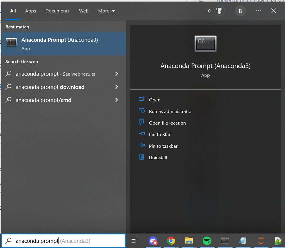
Fig. 10 Open Anaconda prompt.¶

Fig. 11 Type out the install code.¶

Note

When installing packages within a Jupyter Notebook, an exlamation mark is needed to activate pip within the Notebook enviroment. When installing from the command line this is not needed. For example:

!pip install pandas

Exercise

Now let’s import the packages. Type the code below in a new cell in your Notebook and run the cell.

# Import the packages
import pandas as pd
from wordcloud import WordCloud
import matplotlib.pyplot as plt

Note

There is a difference between the import statements of the three packages. In the case of pandas and wordcloud we import the whole package. For matplotlib we only want the pyplot module, so we added this explicitly after the package name. This ensures that ony that module is imported. The as plt and as pd statement renames package to a shorter and easier typable code. You will see this used below.

A package can be used in the same way as a function. We will use the pandas package to load data into the Notebook in a way that is digestable for the creation of a wordcloud. Many packages feature multiple functions for data manipulation, calculation or visualisation. The function you wish to use is added after the package name. The package name points Python to the location of the function.

Syntax:

packagename.function(parameters)

Exercise

Type the code below in a new cell in your Notebook and run the cell.

# Read the dataset into Python using pandas
wordcloud = pd.read_csv("data/wordcloud_dataset.csv", header=None, index_col=0, squeeze=True)
# Transform into dictionary for use in the WordCloud
wordcloud_dict = wordcloud.to_dict()
# It is good practice to check if the data is loaded correctly
wordcloud_dict

Note

As you can see, the pandas name ‘pd’ precedes the option read_csv.

Solution

This should have loaded the data into your Notebook. As stated in the comment it is good practice to check what you have loaded. See if the output matches that below.

C:\Users\mirjam\AppData\Local\Temp\ipykernel_4272\1470747503.py:1: FutureWarning: The squeeze argument has been deprecated and will be removed in a future version. Append .squeeze("columns") to the call to squeeze.

  wordcloud = pd.read_csv("data/wordcloud_dataset.csv", header=None, index_col=0, squeeze=True)

{'machine': 1,
 'learning': 1,
 'read': 1,
 'yesterdays': 1,
 'news': 1,
 'how': 3,
 'semantic': 1,
 'enrichments': 1,
 'enhance': 1,
 'study': 1,
 'digitised': 2,
 'historical': 8,
 'newspapers': 4,
 'creating': 1,
 'data': 11,
 'workflows': 2,
 'humanities': 4,
 'research': 4,
 'automatically': 2,
 'extract': 3,
 'text': 4,
 'layout': 2,
 'metadata': 3,
 'information': 2,
 'from': 5,
 'xmlfiles': 2,
 'ocred': 2,
 'texts': 2,
 'greening': 1,
 'digital': 5,
 'writing': 2,
 'multilayered': 1,
 'articles': 1,
 'example': 1,
 'journal': 1,
 'history': 7,
 'are': 2,
 'we': 1,
 'working': 1,
 'with': 3,
 'opening': 1,
 'keynote': 1,
 'modeling': 1,
 'investigating': 1,
 'variation': 1,
 'language': 1,
 'use': 2,
 'communicative': 1,
 'perspective': 1,
 'methods': 2,
 'challenges': 2,
 'types': 1,
 'evidence': 1,
 'twoway': 1,
 'street': 1,
 'between': 1,
 'ai': 1,
 'media': 2,
 'scholars': 1,
 'developing': 1,
 'stories': 1,
 'as': 1,
 'enhanced': 1,
 'publications': 1,
 'open': 2,
 'science': 1,
 'linked': 2,
 'create': 1,
 'fair': 1,
 'corpus': 1,
 'intra': 1,
 'belgian': 1,
 'literary': 3,
 'translations': 1,
 '19702020': 1,
 'extracting': 1,
 'providing': 1,
 'online': 1,
 'access': 1,
 'annotated': 1,
 'semantically': 1,
 'enriched': 1,
 'agoda': 1,
 'project': 1,
 'moving': 1,
 'beyond': 1,
 'tooloriented': 1,
 'teaching': 1,
 'within': 1,
 'challenge': 1,
 'appropriating': 1,
 'clariah': 1,
 'suite': 1,
 'into': 2,
 'toolsupported': 1,
 'network': 1,
 'analysis': 2,
 'wikipedia': 1,
 'editors': 1,
 'engagement': 1,
 'interests': 1,
 'identities': 1,
 'power': 1,
 'hierarchy': 1,
 'key': 1,
 'actors': 1,
 'events': 1,
 'discourses': 1,
 'gormanrijneveld': 1,
 'translation': 1,
 'controversy': 1,
 'twitter': 1,
 'dragen': 1,
 'van': 1,
 'mondkapjes': 2,
 'niet': 1,
 'nodig': 1,
 'is': 2,
 'zijn': 1,
 'verplichthow': 1,
 'netherlands': 1,
 'dealt': 1,
 'first': 1,
 'wave': 1,
 'covid19': 1,
 'pandemic': 1,
 'promising': 1,
 'road': 1,
 'automatic': 1,
 'speech': 1,
 'recognition': 1,
 'privacysensitive': 1,
 'dutch': 4,
 'doctorpatient': 1,
 'consultation': 1,
 'recordings': 1,
 'understanding': 1,
 'bias': 3,
 'through': 2,
 'datadriven': 1,
 'digitisation': 1,
 'enrichment': 1,
 '100000': 1,
 'pages': 1,
 'handwritten': 1,
 'police': 1,
 'reports': 1,
 'antwerp': 1,
 '18291945': 1,
 'extraction': 1,
 'classification': 1,
 'stamp': 1,
 'cards': 1,
 'using': 2,
 'computer': 1,
 'vision': 1,
 'unlocking': 1,
 'web': 1,
 'archives': 2,
 'seed': 1,
 'lists': 1,
 'derived': 1,
 'defying': 1,
 'expectations': 1,
 'stylistically': 1,
 'unconventional': 1,
 'anger': 1,
 'contemporary': 1,
 'novel': 1,
 'clip': 1,
 'analyze': 1,
 'images': 1,
 'family': 1,
 '3000': 1,
 'dutchlanguage': 1,
 'childrens': 1,
 'books': 1,
 '18001940': 1,
 'distant': 2,
 'reading': 1,
 'gender': 1,
 'prizes': 1,
 'claudine': 1,
 'at': 2,
 'workshop': 1,
 'impact': 1,
 'willy': 1,
 'his': 1,
 'secretaries': 1,
 'colettes': 1,
 'shape': 1,
 'doubt': 1,
 'employing': 1,
 'visualization': 1,
 'investigate': 1,
 'stylistic': 1,
 'features': 1,
 'narrative': 1,
 'works': 1,
 'italo': 1,
 'calvino': 1,
 'unmixing': 1,
 'remix': 1,
 'publishing': 1,
 'complete': 1,
 'manuscripts': 1,
 'anne': 1,
 'frank': 1,
 'zortify': 1,
 'round': 1,
 'table': 1,
 'hybrid': 1,
 'knowledge': 1,
 'new': 2,
 'insights': 1,
 'augmented': 1,
 'intelligence': 1,
 'human': 1,
 'decisionmaking': 1,
 'user': 1,
 'demand': 1,
 'supporting': 1,
 'advanced': 1,
 'collections': 2,
 'exploring': 1,
 'setting': 1,
 'an': 1,
 'agenda': 1,
 'historic': 1,
 'machines': 1,
 'prams': 1,
 'parliament': 1,
 'avenues': 1,
 'collaborative': 1,
 'linguistic': 1,
 'clash': 1,
 'colorful': 1,
 'worlds': 1,
 'viewing': 1,
 'color': 1,
 'western': 1,
 'visual': 1,
 'representations': 1,
 'orient': 1,
 'occident': 1,
 '1890': 1,
 '1920': 1,
 'cutting': 1,
 'its': 1,
 'joints': 1,
 'computational': 1,
 'approach': 2,
 'periodizing': 1,
 'concept': 1,
 'manuscript': 1,
 'syntactic': 1,
 'tree': 1,
 'long': 1,
 'journey': 1,
 'mathematical': 1,
 'bibliographic': 1,
 'textual': 1,
 'studies': 1,
 'personal': 1,
 'library': 1,
 'medieval': 1,
 'sweden': 1,
 'reference': 1,
 'work': 1,
 'transformed': 1,
 'xml': 1,
 'whose': 1,
 'i': 1,
 'it': 1,
 'anyway': 2,
 'comparing': 2,
 'rulebased': 1,
 'bert': 1,
 'token': 1,
 'classifier': 1,
 'quote': 1,
 'detection': 1,
 'whats': 1,
 'liberal': 1,
 'newspaper': 1,
 'performance': 1,
 'usability': 1,
 'stateoftheart': 1,
 'ocr': 1,
 'frenchdutch': 1,
 'bilingual': 1,
 'sources': 1,
 'detecting': 1,
 'perspectives': 1,
 'population': 1,
 'subgroups': 1,
 'pillarised': 1,
 'contentious': 1,
 'words': 1,
 'represented': 1,
 'museum': 1,
 'collection': 1,
 'montage': 1,
 'towards': 1,
 'coherence': 1,
 'multimodal': 1,
 'representation': 1,
 'enriching': 1,
 'cultural': 2,
 'heritage': 1,
 'quest': 1,
 'interoperability': 1,
 'audiovisual': 1,
 'digitized': 1,
 'natural': 1}

When the data is loaded correctly we can use the WordCloud and matplotlib packages to create a wordcloud from the data.

Exercise

Copy the code below in a new cell in your Notebook and run the cell.

# initialise the wordcloud
wc = WordCloud(background_color="white", max_words=20)
# generate the wordcloud 
wc.generate_from_frequencies(wordcloud_dict)
# plt the wordcloud to the output
plt.figure()
plt.imshow(wc,interpolation="bilinear")
plt.axis("off")
plt.show()

Solution

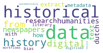
This should plot a wordcloud showing maximally 20 word in different sizes. Each word is sized by the amount of times it occurs in the titles of the DHBenelux 2022 abstract. Common words like ‘the’ and ‘of’ have already been removed. This visualiation can give quick insight to which items are popular at the moment.

Well done! Now you know the basics of working with Jupyter Notebooks and Python. We will use this in the coming chapters.

Automatically extract XML content with Python

1. Introduction to Python and Jupyter Notebooks

Contents

1. Introduction to Python and Jupyter Notebooks¶

Notebooks¶

How does a Notebook work?¶

Different cell types¶

Running cells¶

Adding new cells¶

Comments¶

Python¶

Input and variables¶

Output¶

Functions¶

Conditional statements, if else¶

Packages¶